Optimal Elevator Placement

Published on Sun 22 March 2026

We ask at which floors we should place a set of idle elevators in a building so as to minimize the expected wait time of the next caller. If there is just one elevator, we show that it should be placed at the "median of the demand distribution" — i.e., it should sit at the floor at which half the demand lies above that floor and half below. When there are multiple elevators available, they should be placed at floors such that they each individually sit at the demand medians of their respective "domains". We can use gradient descent to find the solution, but the system is not always convex and so there may sometimes be local minima.

Problem setup – expected wait time

Consider a building with some elevators that customers use to move between floors. We'll assume that demand arrives randomly with distribution

\begin{equation} p(i) = \text{probability next elevator request appears on floor } i \tag{1}\label{1} \end{equation}

If there are \(N\) floors total, then the full set of probabilities can be written as

\begin{equation} \vec{p} \equiv (p_1, p_2, \ldots, p_N) \tag{2}\label{2} \end{equation}

with the \(\{p_i\}\) summing to \(1\). If an idle elevator sits at floor \(j\) and is called to floor \(i\), we posit the rider will have to wait a time

\begin{equation} \text{wait time}(i, j) \equiv |i - j|. \tag{3}\label{3} \end{equation}

for the elevator to arrive. Here, we are choosing some convenient units so that the time to move one floor is exactly one unit of time. The form (\ref{3}) simply says that it takes twice as long for an elevator to get to a location twice as far away.

Question: Where should we place our available idle elevators so as to minimize the expected wait time for the next caller?

Single elevator

If there is just one elevator available, the wait time is minimized if we place it at the median of (\ref{2}). Proof:

If the idle elevator sits at \(j\), the average wait time is

\begin{equation} E(\text{wait time}) = \sum_{i=1}^{N} p(i) |i - j| \tag{4}\label{4} \end{equation}

Differentiating the above wrt \(j\) and setting the result to zero we get

\begin{equation} \partial_j \, E(\text{wait time}) = \sum_{i:\, i \leq j} p(i) - \sum_{i:\, i > j} p(i) = 0\tag{5}\label{5} \end{equation}

The minimum will occur at that point \(j\) where half the weight is below \(j\) and half above — the median of the distribution.

Example 1: simple steady state

Suppose the riders primarily use the elevator to go up from the ground floor to a single upper floor, and then on exit return back to the first floor. In this case, half of all rides start at the ground floor, and the others start on one of the remaining floors \((2, 3, \ldots, N)\). Since exactly half the demand is at floor 1, the median of (\ref{2}) is between floors 1 and 2. We can place the elevator at either location (i.e., floor 1 or 2) to minimize the expected wait time.

Example 2: simple, but up and down demand varies throughout day

Now instead suppose that early in the day more people enter the building, while at the end more people leave. In this case, (\ref{2}) will have more than half its weight at floor 1 at the start of the day. During these periods we should definitely hold the elevator at floor 1. Later in the day, the distribution will shift to having less than half its weight at floor 1 and its median will be on some upper floor.

In a simple case, suppose all people enter at the start of the day and leave at the end of the day. If the upper floors are evenly populated, we then want to hold the elevator in the middle of floors \((2, 3, \ldots, N)\) in the evening — i.e., at floor \(1 + \frac{N}{2}\).

Multiple elevators

To understand the optimal placement of multiple elevators, we'll next pursue a gradient descent type solution. To that end, consider the change in expected wait time when the \(i\)-th elevator moves up a bit to \(x_i \to x_i + \Delta x_i\). As shown in Figure 1, when this occurs the points that this elevator is responsible for have their wait times change. To first order, the effect is

\begin{equation} \Delta E(\text{wait time}) = \Delta x_i \left[ \int_{\frac{x_{i-1}+x_i}{2}}^{x_i} p(x) \, dx - \int_{x_i}^{\frac{x_i+x_{i+1}}{2}} p(x) \, dx \right] \tag{6}\label{6} \end{equation}

That is, the points above ("in front") of \(x_i\) (and served by this elevator) have their wait times reduced by \(\Delta x_i\), while those behind it have their wait times increased by \(\Delta x_i\).

Rearranging (\ref{6}) gives

\begin{equation} \frac{\partial E(\text{wait time})}{\partial x_i} = \int_{\frac{x_{i-1}+x_i}{2}}^{x_i} p(x) \, dx - \int_{x_i}^{\frac{x_i+x_{i+1}}{2}} p(x) \, dx, \tag{7}\label{7} \end{equation}

analogous to (\ref{5}) above. The result (\ref{7}) allows us to apply gradient descent to find the minimum: We start at some convenient initial locations for the idle elevators, use (\ref{7}) to calculate the gradient wrt to their locations, nudge in that direction, and then iterate till convergence. At the minimum, the gradient (\ref{7}) will be zero, implying that each elevator will sit at the median of its "domain" (regions where it is the closest elevator).

Unfortunately, this system is not necessarily convex (see appendix), suggesting gradient descent may sometimes result in finding local, rather than global, minima.

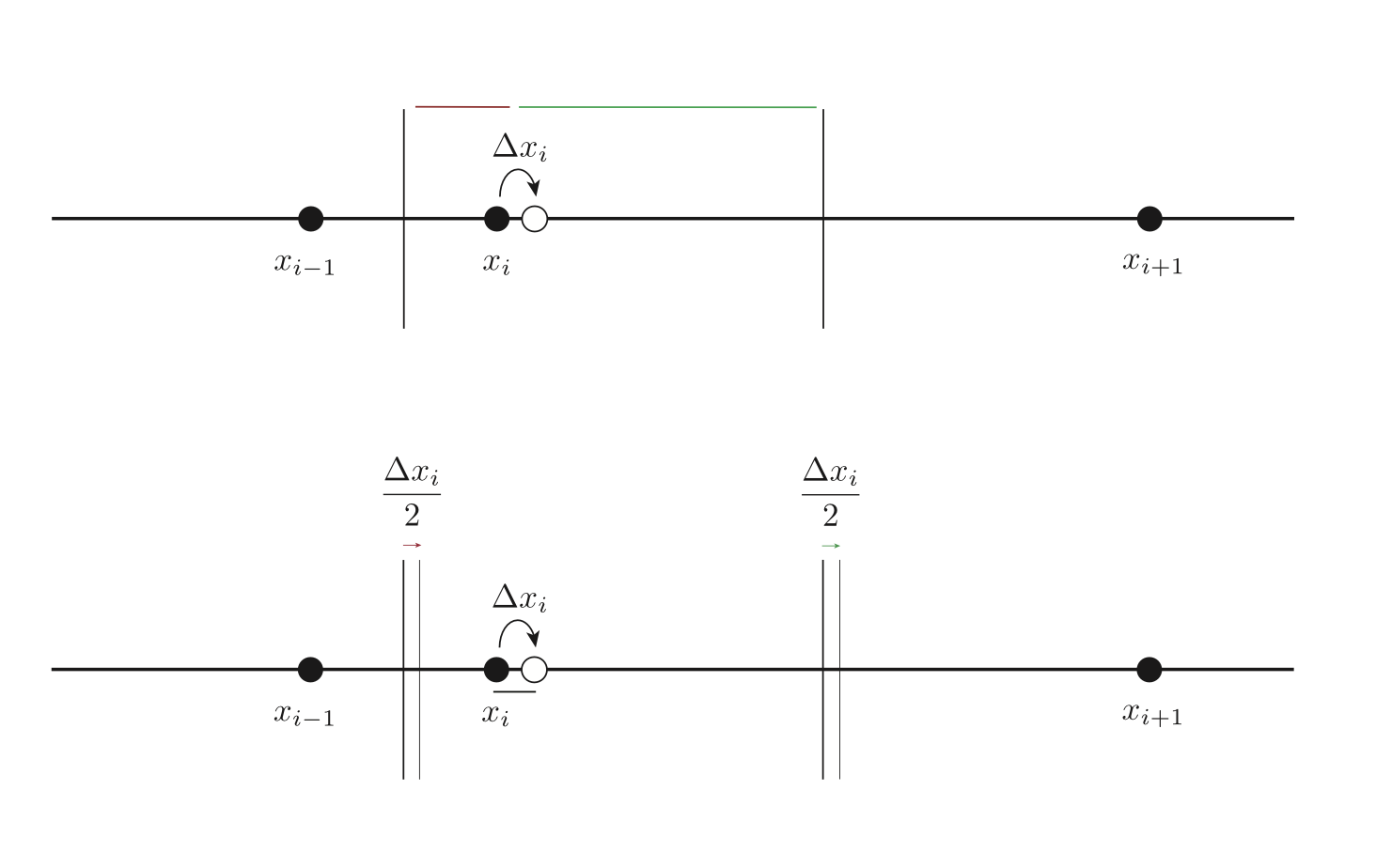
Figure 1: Elevators sit at the locations shown. To minimize wait time, the closest elevator to a demand event is assigned the ride. (top) Here, we illustrate the first derivative of the expected wait time wrt the \(i\)-th elevator's location. At this order what happens is that the floors in front of \(x_i\) have their wait time reduced by \(\Delta x_i\), while those behind have their waits increased by \(\Delta x_i\). (bottom) Here, we consider the second order effects — these are worked out in detail in the appendix: First, the decision boundary changes a bit on either side. At the right, the wait times are reduced, while at the left they are increased. Similarly the little region of width \(\Delta x_i\) right in front of \(x_i\) contributes no net effect to the wait time, but the first order estimate assumes that this region has a reduced wait time. We must correct that, giving an additional positive second order effect. Depending on the demand distribution values at these three points, the net second order effect can be either positive or negative, implying the system is not necessarily convex for all problems.

Appendix: Second order effects

Here, we work out the second order effects from moving the \(i\)-th elevator by \(\Delta x_i\) — we find that this contribution need not always be positive, implying the system is not always convex.

First, consider the "right" boundary between \(x_i\) and \(x_{i+1}\). When we adjust \(x_i\) by \(\Delta x_i\), this boundary will shift to the right by \(\Delta x_i / 2\) as in the bottom of Figure 1. The average wait time for these points before was the time it took the elevator at \(x_{i+1}\) to reach them. Now these points are served by the elevator at \(x_i\). The improvement in expected wait time is

\begin{align} \Delta E(\text{wait time, right boundary}) &= \int_{\frac{x_i+x_{i+1}}{2}}^{\frac{x_i+x_{i+1}}{2}+\frac{\Delta x_i}{2}} \left[(x - x_i - \Delta x_i) - (x_{i+1} - x)\right] p(x) \, dx \nonumber \\ &= - p\!\left(\frac{x_i+x_{i+1}}{2}\right) \cdot \frac{\Delta x_i^2}{2} + O(\Delta x_i^3) \tag{8}\label{8} \end{align}

Here, we've approximated the integral as the domain width times the average value of the integrand over the domain.

Similarly, the points at the left domain edge have their wait times increase. This contributes a term

\begin{equation} \Delta E(\text{wait time, left boundary}) = p\!\left(\frac{x_{i-1}+x_i}{2}\right) \cdot \frac{\Delta x_i^2}{2} + O(\Delta x_i^3) \tag{9}\label{9} \end{equation}

Finally, in the first order estimate we assumed that all points in front of \(x_i\) have their wait times reduced. But the average wait time in the little region of width \(\Delta x_i\) does not change (to lowest order) when we move \(x_i\). We need to remove its contribution from (\ref{6}), giving a term

\begin{equation} \Delta E(\text{wait time, central}) = p(x_i) \, \Delta x_i^2 \tag{10}\label{10} \end{equation}

Combining these terms we see a second order contribution

\begin{equation} \Delta E(\text{wait time, second order}) = \Delta x_i^2 \cdot \left[- \frac{p\!\left(\frac{x_i+x_{i+1}}{2}\right)}{2} + \frac{p\!\left(\frac{x_{i-1}+x_i}{2}\right)}{2} + p(x_i)\right] \tag{11}\label{11} \end{equation}

Depending on the demand distribution \(\vec{p}\), this need not always be positive. We conclude that gradient descent may sometimes result in getting stuck in local minima.