PCA stretch asymptotics

Published on Tue 25 August 2026

This is a companion article to our post PCA response to scaling. There we looked at how the eigensystem of a data set's correlation matrix responds to continuously stretching or compressing a single coordinate direction. We showed that the eigenvalues always maintain their relative order under such transformations. Here, we present a few additional calculations relating to the asymptotics of this system:

We work out the exact asymptotic (limiting) forms of the eigenvalues and eigenvectors in the two extreme single-axis scaling regimes: a very strong compression (\(s \ll 1\)) and a very strong stretch (\(s \gg 1\)) along a single direction.
We show that one can start with any covariance matrix and map it to any other of the same dimension via a finite series of single-axis scalings.
We integrate the perturbation equations in the limit of a near-crossing of two eigenvalues. This provides a "microscopic" view of the eigenvector rotation effect described in our other post.

In addition to these results, we present a simple general result on the determinant of the scaled covariance matrix in an appendix.

Limiting single-axis scaling forms

Strong compression limit

Asymptotic algebraic solution

We begin by considering what happens when we compress by \(s \ll 1\) along the \(x\) direction. It is helpful to write the covariance matrix in block form,

\begin{equation} M \equiv \begin{pmatrix} s^2 a & s\, \vec b^{\,T} \\ s\, \vec b & C \end{pmatrix} \tag{1}\label{1} \end{equation}

with \(a \equiv M_{11}\), etc. The eigensystem satisfies

\begin{equation} s^2 a\, x + s\, \vec b^{\,T} \cdot \vec y = \lambda x \tag{2}\label{2} \end{equation}

\begin{equation} s\, \vec b\, x + C \cdot \vec y = \lambda \vec y \tag{3}\label{3} \end{equation}

Looking for a small eigenvalue with \(x \sim 1\) and \(y \sim O(s)\), the first equation suggests the eigenvalue will be \(O(s^2)\). In the second equation then, the left two terms dominate, and we get

\begin{equation} \tag{4}\label{4} s \vec{b} x + C \vec{y} \sim 0, \end{equation}

\begin{equation}\tag{5}\label{5} \vec{y} \sim - s C^{-1} \cdot \vec{b} \end{equation}

Plugging into the first eigenvalue equation then gives

\begin{equation} s^2 a\, x - s^2\, \vec b^{\,T} \cdot C^{-1} \cdot \vec{b} x = \lambda x \tag{6}\label{6} \end{equation}

\begin{equation} \tag{7}\label{7} \lambda \sim s^2 \left (a - \vec b^{\,T} \cdot C^{-1} \cdot \vec{b} \right) \end{equation}

The eigenvalue indeed vanishes like \(s^2\).

Next, we look for the remaining \(n-1\), finite eigenvalues. Here \(x\) must go to zero as \(s \to 0\) in order to maintain mode orthogonality. Balancing \(\lambda x\) against \(s\, \vec b^{\,T} \cdot \vec y\) in (\ref{2}) (the \(s^2 a x\) term is subleading here), we get \(x \sim (s / \lambda)\, \vec b^{\,T} \cdot \vec y\). Plugging into (\ref{3}),

\begin{equation} \left(C + O(s^2)\right) \cdot \vec y = \lambda \vec y \tag{8}\label{8} \end{equation}

To leading order then, the finite eigenvalues and eigenvectors are simply those of \(C\) — the correlation matrix of the data with the compression direction dropped entirely. We used this result in a key step of the sister post.

Geometric interpretation

After a strong compression along \(\textbf{e}_1\), the finite eigenvalues and eigenvectors above are simply those of the space orthogonal to \(\textbf{e}_{1}\). This is easy enough to understand. How can we interpret (\ref{7}), the eigenvalue of the compressed component?

What's happening here is illustrated in Figure 2 below, for a simple 2-d case. When we compress strongly along \(\textbf{e}_1\), one eigenvector will be nearly parallel to this compressed direction. The eigenvalue corresponding to this direction will be the squared variance of the data along this direction. In other words, it will be the variance of the distance to the space spanned by the other eigenvector for each point. We've drawn that distance in solid black below, and have also drawn the \(x\)-distance to the larger eigenvector using a dashed line.

At left we see the original space, and at right the compressed space. Notice that in the compressed space the solid and dashed lines begin to align because the lowest principal component is now nearly parallel to \(\textbf{e}_1\). In the limit of very strong compressions then, the distance to this subspace will simply be its \(\Delta x\) value. In other words, we need to know the \(x\) value for a given data point, as well as the \(x\) value of the space spanned by the finite principal components at fixed \(\vec{y}\). At strong compressions, this turns out to be the \(x\) value obtained through linear fit onto the other data points. This gives,

\begin{eqnarray} \label{9} \tag{9} \Delta x_i &=& x_i - \vec{b}^T \cdot C^{-1} \cdot \vec{y}_i, \\ &\equiv& x_i - \vec{\beta} \cdot \vec{y}_i. \end{eqnarray}

The variance of the \(\Delta x_i\) values is then

\begin{eqnarray} \tag{10}\label{10} \text{var} (\Delta x) &\equiv& s^2 (1, - \vec{\beta})^T \cdot M \cdot (1,- \vec{\beta}) \\ &=& s^2 \left ( M_{11} - \vec{b}^T \cdot C^{-1} \cdot \vec{b} \right), \end{eqnarray}

agreeing with (\ref{7}). In other words, the width of the smallest component is not just the width in \(x\), but the distance to the space spanned by the other components, and this is what gives the correction shown in (\ref{7}).

Compressed along x

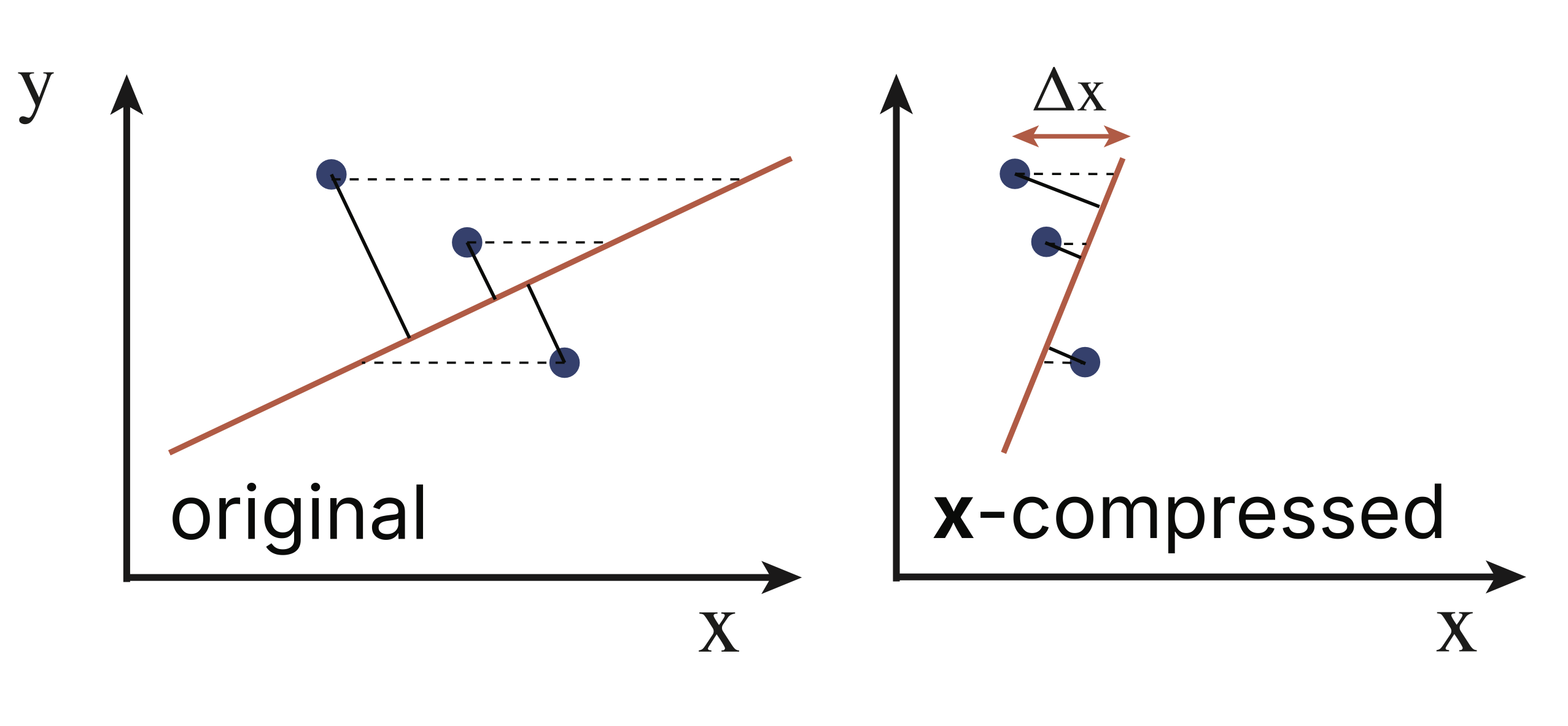
Figure 2: Under a strong compression, the distance of a data point to the space spanned by the finite eigenvalue principal components approaches its \(x\)-distance (the dark and dashed lines approach each other in the right figure). If we project out the part of the data explained by the other components, we then get the residual \(x_1 - f_{x_1}(x_2, x_3, \ldots)\), where \(f_{x_1}(x_2, x_3, \ldots)\) is the linear regression of \(x\) on the other components. Including the \(s^2\) compression, this has variance as given in (\ref{7}).

Strong stretch limit

Algebraic solution

Let's now look for the solutions to (\ref{2}) and (\ref{3}) in the strong stretch limit, \(s \gg 1\). If we look for a large eigenvalue, the first of these equations gives

\begin{equation} x \sim 1, \quad \lambda \sim s^2 a\; (\equiv s^2 M_{11}). \tag{11}\label{11} \end{equation}

Plugging (\ref{11}) into the second equation, we get

\begin{equation} \vec y \sim \frac{1}{s\, a}\, \vec b \tag{12}\label{12} \end{equation}

The equations (\ref{11}) and (\ref{12}) give the principal component to leading order in \(s\). The eigenvalue in this case is simply the net variance in the \(x\) direction after stretching.

Next, we look for the finite eigenvalues. We know \(x\) won't be large for these, so neither will be \(\lambda x\), and the first eigenvalue equation (\ref{2}) goes to

\begin{equation} (s^2 a)\, x + s\, \vec b^{\,T} \cdot \vec y = 0 \quad \to \quad x = -\frac{\vec b^{\,T} \cdot \vec y}{s\, a} \tag{13}\label{13} \end{equation}

Plugging into the second equation (\ref{3}), we get

\begin{equation} \left(C - \frac{1}{a}\, \vec b\, \vec b^{\,T}\right) \cdot \vec y = \lambda \vec y \tag{14}\label{14} \end{equation}

This gives the eigensystem for the finite eigenvalues at large \(s\). We see there are again \(n - 1\) finite solutions of \(O(1)\). However, unlike in the strong compression case, the finite eigensystem is not simply that of \(C\).

Geometric interpretation

In the figure below, we give a geometric interpretation of what's happening with respect to the finite eigenvalues: In short, at large \(s\) the data orthogonal to the first principal component is that part not explained by a linear fit to the data, regressing \(y_i\) on \(x\). The slope of the fit (in the unstretched system) of \(y_i\) to \(x\) is given by \(m \equiv \frac{M_{xy_i}}{M_{xx}}\), so the data in that direction gets mapped to

\begin{equation} \widetilde y_i \equiv y_i - \frac{M_{1i}}{M_{11}}\, x \tag{15}\label{15} \end{equation}

The covariance of \(\widetilde y_i\) and \(\widetilde y_j\) is then

\begin{equation} \widetilde M_{ij} = \left(\widehat e_i - \frac{M_{1i}}{M_{11}}\widehat e_1\right)^T \cdot M \cdot \left(\widehat e_j - \frac{M_{1j}}{M_{11}}\widehat e_1\right)^T = M_{ij} - \frac{M_{i1}M_{1j}}{M_{11}}, \tag{16}\label{16} \end{equation}

which is equivalent to the left side of (\ref{14}).

Stretched along x

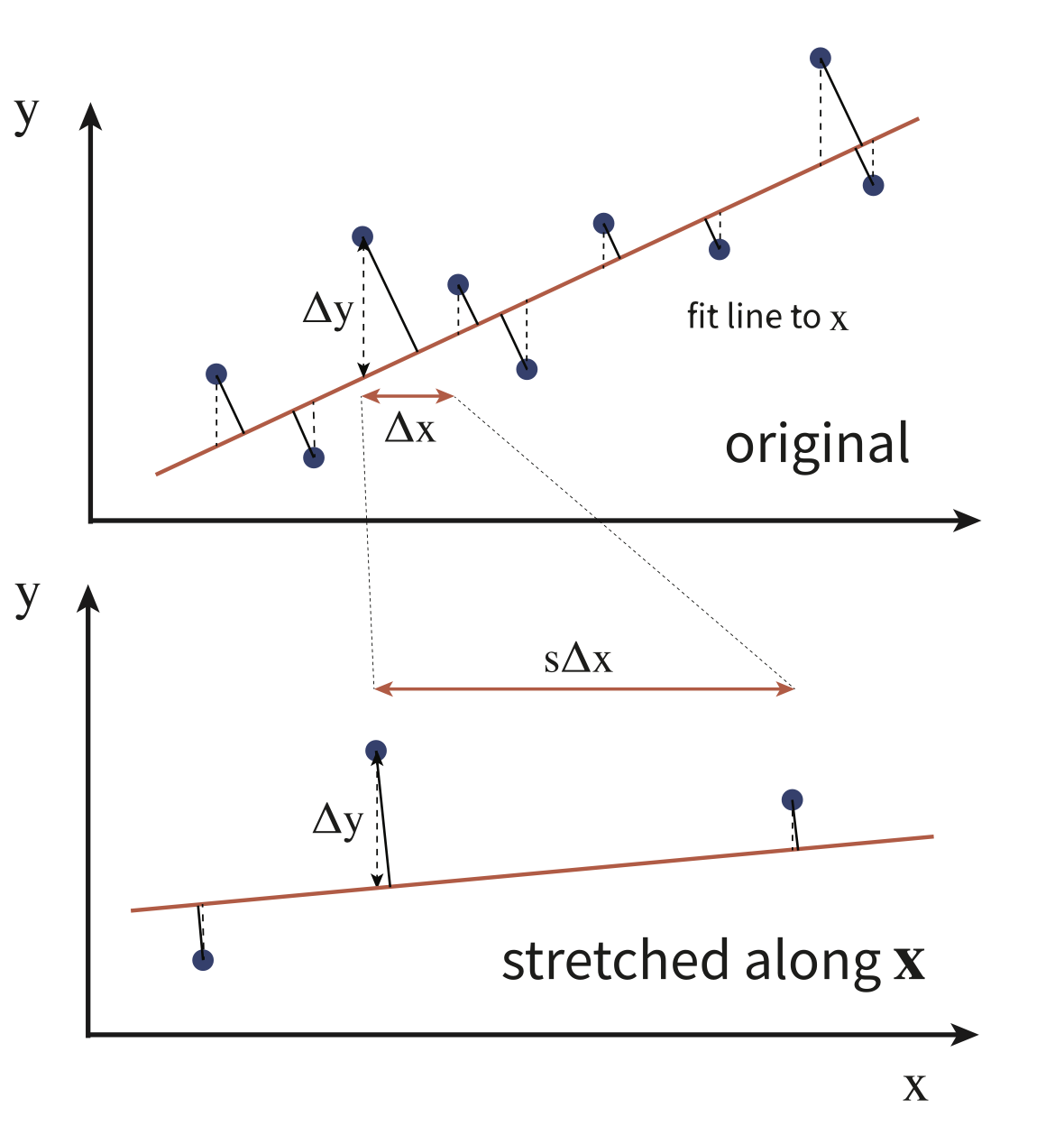
Figure: Plots of one component \(y\) vs \(x\) — the direction along which we stretch: (top) original system, (bottom) stretched system. First notice that the data to be explained by the second and lower principal components is that part remaining once we project orthogonally to the first component. Next, we note that when we stretch strongly, the first principal component aligns with the linear regression of \(y\) vs \(x\) (e.g., see our prior post on PCA vs regression slopes), which in turn rotates to be close to parallel to \(\widehat x\). In this limit, the orthogonal projection off the first component (solid black projection lines) ends up reducing to the \(y\)-distance to the fit line (dashed projection lines). This dashed projection is the same as that in the unstretched system, and so the \(y\) data gets mapped to \(\Delta y \equiv y - \frac{M_{12}}{M_{11}}\, x\), the original value of \(y\) minus the value of \(y\) along the regression of \(y\) vs \(x\).

Mapping between covariance matrices

Algebraic solution

In our main post, we demonstrated that eigenvalue ordering is maintained when scaling along single axis directions. We then argued that this implies that ordering is maintained for any scaling transformation, since these can always be carried out via a series of single-axis scalings. Here, we spell this latter point out.

The first observation to make is that any positive definite matrix can be considered a set of scalings. To see this, consider the matrix in the basis of its eigenvectors. In that frame, the transformation can be seen to be diagonal with a separate scaling factor for each direction.

Now, whenever we transform via a scaling, an initial covariance matrix will be mapped into some new covariance matrix. We can then identify the set of possible scalings by first identifying all covariance matrices that an initial one can be mapped into. Assuming our initial matrix is positive definite, we can easily see that this is the full set of other positive definite matrices. Indeed, ChatGPT was able to quickly write down the following transformation: Let \(M\) be our initial matrix and \(T\) be our target. If we then write

\begin{equation} S = M^{-1/2} \left( M^{1/2} T M^{1/2} \right)^{1/2} M^{-1/2}. \tag{17}\label{17} \end{equation}

then one can easily see that this is a real symmetric positive definite matrix, and also that

\begin{equation} T = S \cdot M \cdot S \tag{18}\label{18} \end{equation}

That is, we have a finite set of scalings (along the \(n\) eigenvectors of \(S\)), that maps \(M\) to \(T\).

This is striking, given the result from our main post that the eigenvalues maintain their order through any scaling transformation. Combining that with this result, we see that any pair of covariance matrices can be mapped from one to the other via a finite set of scalings, at each step maintaining eigenvalue order.

Geometric solution

Before moving on, we give an alternative, geometric method to map between any two covariance matrices, this time motivated by our asymptotic results above. In order to map from one covariance to another, we will proceed one eigenvector at a time. Once we get one eigenvector to align with a target direction, we can work in the subspace orthogonal to that to align the next eigenvector, etc.

To align the first eigenvector of \(M\) with that of \(T\), recall that in the limit of a strong compression, the smallest eigenmode rotates to align with that direction. In the limit of a very strong compression, (\ref{9}) gives the part of this vector that is orthogonal to the compression direction (taken as \(\textbf{e}_1\) here for simplicity). What one can do then to align an eigenmode with the target direction is to first compress strongly along the target direction, and then follow up by stretching back out along the final eigenmode's direction (taking into account the small bit left orthogonal to the compression direction of the smallest mode when it is compressed). Working through the asymptotics, the combined effect of these two steps is easily found to be

\begin{equation} S = \begin{pmatrix} 1 & -\mathbf{b}^T C^{-1} \\ \mathbf{0} & I \end{pmatrix} \tag{19}\label{19} \end{equation}

Applying the pair of scalings to \(M\) then gives

\begin{equation} S M S^T = \begin{pmatrix} m_{11} - \mathbf{b}^T C^{-1} \mathbf{b} & \mathbf{0}^T \\ \mathbf{0} & C \end{pmatrix}. \tag{20}\label{20} \end{equation}

and the first mode is now aligned with the target direction. Applying an extra factor to the second scaling step we can also adjust the eigenvalue as desired. Again, continuing in this way we can align each of the other modes as well.

Near-crossings

Using the perturbation equations for \(d\lambda_i/ds\) and \(d \vec{v}_i/ds\) derived in the main post (equation (6) there, together with equation (7) dotted with \(\widehat e_1\) to isolate the evolution of \(\alpha_i \equiv \widehat e_1 \cdot \vec v_i\)), we can obtain an algebraic view of what happens in a generic system that is close to a near eigenvalue crossing.

To simplify the equations, we first change variables to

\begin{equation} t \equiv 2 \log s, \qquad dt = \frac{2}{s}\, ds, \tag{21}\label{21} \end{equation}

\begin{equation} p_i \equiv \alpha_i^2. \tag{22}\label{22} \end{equation}

Plugging these into the perturbation equations gives

\begin{equation} \frac{d\lambda_i}{dt} = \lambda_i\, p_i \tag{23}\label{23} \end{equation}

\begin{equation} \frac{dp_i}{dt} = p_i \sum_{j \neq i} \frac{\lambda_i + \lambda_j}{\lambda_i - \lambda_j}\, p_j \tag{24}\label{24} \end{equation}

Suppose the eigenvalues are initially non-degenerate and ordered as \(\lambda_1 < \lambda_2 < \ldots < \lambda_n\). Consider then whether two adjacent eigenvalues, \(\lambda_i\) and \(\lambda_{i+1}\), can cross at some point in the evolution with respect to \(t\). From (\ref{23}), the growth of \(\lambda_i\) is proportional to \(\lambda_i\) itself, a term that will tend to support order maintenance. However, that growth is also proportional to \(p_i\), and it's possible to have \(p_i > p_{i+1}\) at the start — suggesting the lower eigenvalue might initially grow faster than the larger one.

Suppose we sit at a point where two adjacent eigenvalues are close. Let

\begin{equation} \lambda_{i+1} \equiv \lambda + \frac{\Delta}{2}, \qquad \lambda_i \equiv \lambda - \frac{\Delta}{2}, \qquad \Delta \equiv \lambda_{i+1} - \lambda_i \ll 1, \tag{25}\label{25} \end{equation}

\begin{equation} q \equiv p_{i+1} - p_i, \qquad m \equiv p_{i+1} + p_i. \tag{26}\label{26} \end{equation}

We'll show that \(\Delta\) must stay positive. Plugging these definitions into (\ref{23}) and (\ref{24}) and keeping terms only to lowest order in \(\Delta\) gives

\begin{equation} \frac{d\Delta}{dt} = \lambda q + O(\Delta) \tag{27}\label{27} \end{equation}

\begin{equation} \frac{dq}{dt} = \frac{\lambda}{\Delta}\left(m^2 - q^2\right) \tag{28}\label{28} \end{equation}

\begin{equation} \frac{dm}{dt} = O(1) \tag{29}\label{29} \end{equation}

The second of these equations, (\ref{28}), tells us that as \(\Delta \to 0\), weight along \(\widehat x\) shifts rapidly from the lower component to the upper one. This is what brings us to the regime where both terms on the right of (\ref{23}) act together to support order maintenance. Indeed, dividing (\ref{27}) by (\ref{28}) gives

\begin{equation} \frac{d\Delta}{dq} = \frac{\Delta \cdot q}{m^2 - q^2}, \tag{30}\label{30} \end{equation}

Since \(m\) changes only at \(O(1)\) in \(t\) — much more slowly than \(q\) does as \(\Delta \to 0\) — we can treat \(m\) as fixed and integrate this line directly, giving

\begin{equation} \Delta^2 \left(m^2 - q^2\right) = C, \tag{31}\label{31} \end{equation}

with \(C\) a constant, to lowest order in \(\Delta\).

This conservation law is what implies order maintenance: if \(\Delta\) is close to zero and attempts to get closer still, the second factor in (\ref{31}), \(m^2 - q^2\), must grow quickly to compensate and maintain the conservation law. But \(m^2 - q^2 \equiv O(1)\), and so cannot grow without bound. We conclude that the two eigenvalues cannot get arbitrarily close — and so cannot cross — if (\ref{31}) is to be maintained.

How small can \(\Delta\) get? We can rewrite (\ref{31}) as

\begin{equation} 4 \Delta^2 p_i p_{i+1} = C, \tag{32}\label{32} \end{equation}

Now from (\ref{26}), the sum of \(p_i\) and \(p_{i+1}\) is \(m\), which is fixed over the \(t\) time scale (this is the net power along the stretch direction of the two nearly-degenerate modes). The product of the two is therefore maximized when the two are equal (by the arithmetic geometric mean inequality). This gives

\begin{equation} \Delta^2 \geq \frac{C}{m^2} \tag{33}\label{33} \end{equation}

Next we plug (\ref{31}) into (\ref{28}), to obtain

\begin{equation} \frac{dq}{dt} = \frac{\lambda C}{\Delta^3}, \tag{34}\label{34} \end{equation}

This implies a bounce: As the two eigenvalues approach each other, weight along the scaling direction quickly pushes from the lower eigenvalue to the larger throughout. When this occurs, (\ref{27}) implies \(\Delta\)'s growth will also change signs and the two eigenvalues will start to separate. Further, as we enter and exit the bounce, (\ref{31}) tells us the \(q^2\) value must be the same at equal values of \(\Delta\). We do not show this last step here, but a simple asymptotic calculation shows that this implies a swapping of the orientations of the two modes on either side of the bounce, consistent with the "macroscopic" view that we covered in the sister post.

Appendix A: A determinant identity

Here we note a simple constraint on how the eigenvalues of \(M(s)\) can vary as we scale our system. A first observation is that we can write

\begin{equation} M(s) = S\, M\, S \tag{35}\label{35} \end{equation}

where

\begin{equation} S = diag(s, 1, 1, ..., 1). \tag{36}\label{36} \end{equation}

In general, if we scale more than one measurement — perhaps each according to a different scale factor — we'll just need to insert each direction's scale into \(S\). If we scale in only one direction, (\ref{35}) gives

\begin{equation} det\, M(s) = s^2\, det\, M(1) \tag{37}\label{37} \end{equation}

This puts one simple constraint on how the eigenvalues can vary as we scale our system.