PCA slope vs regression slope

Published on Sat 16 May 2026

A regression fit can sometimes look surprisingly poor when plotted on top of data, with the two having visually different slopes. The reason is that the line that visually seems to go through the data best is that which minimizes total projection error, while the least squares fit minimizes squared \(y\)-error at each fixed \(x\) (e.g., see this prior Hacker News thread for discussion). Here, we make these points concrete by working out the exact angular difference between the two fits. We find the effect is strongest when the least squares fit has a slope of \(m = 1/\sqrt{3}\), running \(30\) degrees off the x-axis, as in Figure 1 below.

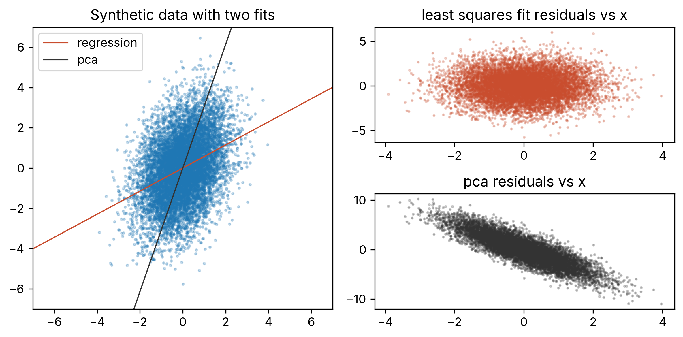
Figure 1: Synthetic data generated from (\ref{1}) with \(m=1/\sqrt{3}\), \(\sigma^2=1\). The regression line (red) minimizes squared vertical residuals, while the PCA line (black) minimizes total squared perpendicular distance. Although the PCA line visually seems to fit the data much better, the plots at right show that the least-squares residuals are uncorrelated with \(x\), while PCA residuals show a clear trend.

Evaluating the slope from the two fits

We'll work here with a simple model where \(y\) is related to \(x\) via slope \(m\) and additive noise:

\begin{equation} y_i = m x_i + \epsilon_i \tag{1}\label{1} \end{equation}

Here, \(\epsilon_i\) has variance \(\sigma^2\). Taking a least-squares fit to plenty of data generated in this way will return a slope of \(m\) and an intercept of \(0\), as expected.

Now, in our prior post on PCA, we reviewed that the PCA direction is the eigenvector corresponding to the largest eigenvalue of the data's covariance matrix. The components of this matrix are as follows: Choosing the scale so that \(E(\delta x^2) = 1\), we have

\begin{equation} E(\delta y^2) = E\!\left[(m\,\delta x_i + \epsilon_i)(m\,\delta x_i + \epsilon_i)\right] = m^2 + \sigma^2 \tag{2}\label{2} \end{equation}

and

\begin{equation} E(\delta x \cdot \delta y) = E\!\left[\delta x \cdot (m\,\delta x_i + \epsilon_i)\right] = m \tag{3}\label{3} \end{equation}

The covariance matrix is then

\begin{equation} C = \begin{pmatrix} 1 & m \\ m & m^2 + \sigma^2 \end{pmatrix} \tag{4}\label{4} \end{equation}

The eigenvalues of \(C\) are

\begin{equation} \lambda_{\pm} = \frac{1 + m^2 + \sigma^2 \pm \sqrt{(1 + m^2 + \sigma^2)^2 - 4\sigma^2}}{2} \tag{5}\label{5} \end{equation}

Again, in PCA we project the data onto the eigenvector corresponding to the larger eigenvalue. This is

\begin{align} v_+ &= \left[1,\; \frac{\lambda_+ - 1}{m}\right] \notag \\ &\sim \left[1,\; m + \frac{m}{1+m^2}\,\sigma^2 + O(\sigma^4) \right] \tag{6}\label{6} \end{align}

where the last line gives the first two terms in the small \(\sigma^2\) limit.

From (\ref{6}), we read out that the PCA slope is given by

\begin{equation} \text{svd slope} \sim m\!\left(1 + \frac{\sigma^2}{1+m^2} + O(\sigma^4)\right) \tag{7}\label{7} \end{equation}

Relative to the regression slope \(m\), this is increased by a scale factor of

\begin{equation} \kappa \equiv 1 + \frac{\sigma^2}{1+m^2} + O(\sigma^4)\tag{8}\label{8} \end{equation}

Maximizing the angular difference

The slope of a line is related to its angle off the \(x\)-axis by

\begin{equation} m = \tan\theta \tag{9}\label{9} \end{equation}

To get the change in angle for our case, we use

\begin{equation} \theta_2 - \theta_1 = \arctan(\kappa m) - \arctan(m) \approx \frac{m}{1+m^2}(\kappa - 1) + O(\kappa-1)^2 \tag{10}\label{10} \end{equation}

Plugging in (\ref{8}), the change in angle is then

\begin{equation} \Delta\theta = \frac{m}{(1+m^2)^2}\,\sigma^2 + O(\sigma^4) \tag{11}\label{11} \end{equation}

The coefficient in front of \(\sigma^2\) is \(\frac{m}{(1+m^2)^2}\), and this is largest at \(m = 1/\sqrt{3}\), where \(\theta = 30\) degrees.