Series Summation Methods
Published on Sun 18 October 2026
Here, we will maintain a list of series summation methods. Methods currently covered:
Method 1: Operator method
The approach was developed by Isaac Newton. It turns series summation into a mechanical process.
Method
Consider a series \(a_0, a_1, \ldots, a_n\). Define two operators \(E\) and \(\Delta\) satisfying
Imagining that the \(\{a_i\}\) are partial sums of some series, we'd like to evaluate
We can make progress by noting that our two operators are related via
Rearranging, and plugging into (\ref{2}), we get
From here, two things can happen: (a) We can clip the expansion at level \(k\) to get a polynomial fit to the series. This is the interpolating polynomial of degree \(k\) that goes through the points \((0, a_0), (1, a_1), \ldots, (k, a_k)\). (b) It may be that \(\Delta^i a_0 = 0\) for all \(i \geq k\), say. In that case, the series is exactly polynomial in \(n\).
Before moving on, we note that we can also expand \(\Delta^n\) in terms of \(E\) using (\ref{3}). This gives
an expression that sometimes provides a convenient way to evaluate the \(n\)-th difference.
Example
Let's evaluate \(a_n = \sum_{i=0}^n i^2\), the sum of the first \(n\) squares. To calculate the first few terms in (\ref{4}) for this series, we'll need to evaluate \(\Delta a_i\) for the first few \(a_i\). These values are
Naturally, we get back the subsequent squares in each case. The second differences are
Finally, the third differences are
We see the last two values are both \(2\). In fact, every term in the third difference sequence is \(2\), so we get
and all higher order differences are zero as well. Plugging these results into (4), we obtain
the familiar result. Notice that the sum of squares is cubic in \(n\), just as the integral of a quadratic gives a cubic.
Method 2: Euler transform for alternating series
Here, we review Euler's method for speeding up the convergence of alternating series. This makes use of the operator identity we reviewed above.
Method
Let \(a_i \geq 0\), and define the alternating series
Here, we have summed the geometric series in the second line. Next, we use (\ref{3}) to obtain
Notice that we have differences appearing here, which often converge more quickly, and the factor of \(2^{-i}\) will also help to speed up convergence. Note also that (\ref{5}) can be used to programmatically evaluate these terms.
Example
Consider the alternating sum
By the Leibniz test, this series converges. However, the logarithm does not grow quickly and so we expect slow convergence here. Indeed, even summing the first 100 million terms, we get an estimate having about 3 percent error. In contrast, with the Euler method we can obtain sixteen-digit accuracy using just \(k\) terms, where
Figure 1 below illustrates the much faster rate of convergence of the Euler-transformed sum in this case.
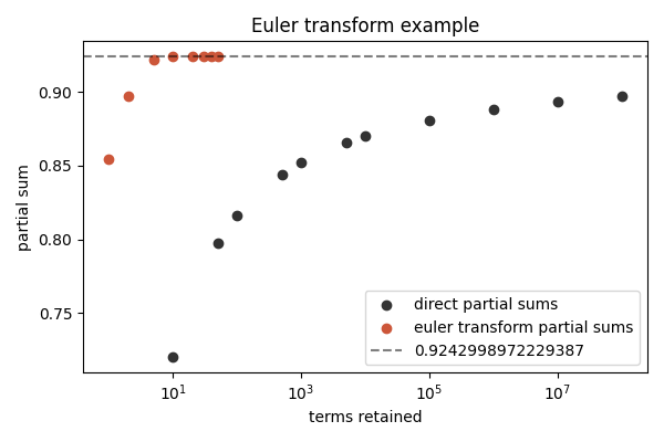
Figure 1: Plot of the partial sums of (\ref{13}) for both the direct and Euler-transformed sums. The direct sum has not converged even after 100 million terms, but the Euler-transformed sum reaches machine precision after just 50.
Method 3: Borel trick
The Borel trick sometimes allows us to assign a "physical" value to a divergent series. We assume the series is the asymptotic expansion of some function that does not have a converging Taylor expansion. It is particularly natural when the \(n\)-th term scales like \(n!\), which indicates zero radius of convergence, perhaps due to a branch cut extending to the origin. There are practical applications of the trick in statistical mechanics and quantum physics, but these are too complicated for this post. Instead, I give a toy example below.
Method
Let
be a series that may or may not converge. Multiply the \(k\)-th term by \(\frac{1}{k!}\) to obtain a new series
Suppose this can be summed, and then we carry out the following integral
This returns \(S(g)\) since the expansion of \(f(gt)\) in (\ref{17}) gives a series of gamma functions, canceling out the introduced factorials in (\ref{16}). To apply the trick, we evaluate the sum first and then integrate.
Example
Let
Applying the first step of our trick, we obtain
Next,
Setting \(g \rightarrow 1\), we get
a familiar expression.
Note that in this case, we didn't actually need the Borel trick since the terms of the series were not growing like the factorials. Indeed, we can obtain this result more simply by introducing the powers of \(g\) alone. For an example where the factorial management is essential, consider the sum \(\sum n! (-g)^n\), which diverges for all \(g\). Here, the Borel trick gives a finite result involving the exponential integral.
Method 4: Shanks transform
The Shanks transform provides a simple method to accelerate the convergence of a series. We assume that the error in the partial sums behaves to leading order like a geometric decay. We then use consecutive partial sums to evaluate the leading error's form and then remove it.
Method
Consider the partial sum
We're interested in evaluating the infinite series
We posit that to leading order
where \(S\), \(A\), and \(r\) are unknown. To estimate these, we consider three consecutive values of \(S_n\),
A bit of simple algebra allows us to solve these equations for \(S\). Writing that estimate for \(S\) as \(S_{Shanks, n}\), we get
The idea of the Shanks transform then is to replace the \(n\)-th partial sum by the corrected form (\ref{26}), which allows us to "peel off" the leading error term. This approximation will become more accurate as we get to larger \(n\), where the asymptotic form will be more accurate. If there are additional error terms, they can often be removed via additional applications of the transform. To do that, we use the first line of (\ref{26}), replacing \(S_n\) by \(S_{Shanks, n}\), etc.
Example
Consider the sum
By eye, we can see that this has the required exponential convergence form that suggests the Shanks transform will be useful. Indeed, in Figure 2 below, I plot the partial sums and their first two Shanks transforms. You can see that the first Shanks transform converges at a faster exponential rate than the original sum, and the second converges faster still. With each successive transform, we can often improve our rate of convergence further.
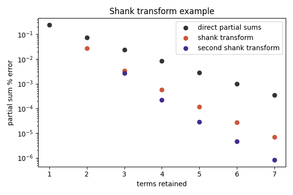
Figure 2: Residual errors in the partial sum of (\ref{27}), as well as those from the Shanks transformed partial sums. The transform allows for convergence at a faster exponential rate. Here, we start the first Shanks transform at \(x=2\), since it requires knowledge of both \(a_1\) and \(a_2\). Similarly, we start the plot of the second transform at \(x=3\), since it requires knowledge of the first three terms.