A scale invariance property of PCA

Published on Tue 25 August 2026

The PCA algorithm is sensitive to changes in measurement scale. Measuring one variable of a system in inches rather than centimeters, say, alters both its principal axes and principal eigenvalues. Although this scale dependence is generally complicated, we show here that it nevertheless obeys a strict invariance property:

Under a continuous scale adjustment, the initial state's \(k\)-th largest principal component (ordered by eigenvalue) continuously evolves into the final state's \(k\)-th largest principal component, for each \(k\). In this sense, we can say that the modes of PCA are "order-stable" with respect to changes in measurement scale — see Figure 1 below for an example.

A special case occurs when scaling along directions that are orthogonal to some modes — here, apparent eigenvalue crossings can occur. However, we show that we can interpret these apparent crossings as cases where the modes instantaneously swap their orientation, in this way maintaining the required order stability.

Figure 1: PCA response to scaling in \(2\)-d: When we compress along the \(\textbf{x}\)-direction, the smaller (black) principal component rotates to align with the compression direction. Similarly, when we stretch, the larger (red) principal component rotates into the stretch direction. At all scales, a consistent eigenvalue ordering is maintained — the black mode is always the smaller of the two and the red is always the larger.

Introduction

In Principal Component Analysis ("PCA" for short, see our prior post for an intro), we are concerned with the eigensystem of a given data set's covariance matrix,

\begin{equation} M = \begin{pmatrix} M_{11} & M_{12} & \ldots \\ M_{21} & M_{22} & \ldots \\ \ldots & & \end{pmatrix} \tag{1}\label{1} \end{equation}

The eigensystem provides us with an ellipsoidal approximation to the data set, giving us a sense of its geometry. Projecting into the space spanned by a truncated subset of these eigenvectors can often give us a high-fidelity compression of the data set. These applications make PCA a workhorse algorithm in data analysis. The fact that its outputs are sensitive to measurement scale is therefore a cause of frequent discomfort: It's almost never clear which choice of units (and which downstream PCA output) is the objectively "right" one for a given application. This motivates our work here, where we aim to better understand the response of PCA to changes in measurement scale.

To focus our attention, we'll be mostly interested here in the response to a simple scaling of the first coordinate, writing \(x \to s\, x\). In this case,

\begin{equation} \langle \delta x, \delta y \rangle \to s\, M_{xy} \tag{2}\label{2} \end{equation}

and

\begin{equation} \langle \delta x^2 \rangle \to s^2\, M_{xx} \tag{3}\label{3} \end{equation}

This sends the covariance matrix to

\begin{equation} M(s) = \begin{pmatrix} s^2 M_{11} & s M_{12} & s M_{13} & \ldots \\ s M_{21} & M_{22} & M_{23} & \ldots \\ s M_{31} & M_{32} & M_{33} & \ldots \\ & \ldots & & \end{pmatrix} \tag{4}\label{4} \end{equation}

How do the eigenvectors and eigenvalues of this matrix change as we adjust the scale factor \(s\)?

Our key result is that the eigenvalues of (\ref{4}) never cross as we vary \(s\), but instead always maintain their order. Because this holds for scaling along any single direction, the result extends to general scalings by composition, one scaling direction at a time. The result can be proved using a strict-interlacing theorem for rank-one perturbations of real symmetric matrices [1]. Here, we instead give a direct proof tailored to the positive-definite real symmetric setting, which also provides a geometric explanation of the result. We first analyze the "generic" case, in three steps:

First-order perturbation theory shows that every eigenvalue increases monotonically with \(s\).
In the limit of a very strong compression (\(s \to 0\)), one eigenvalue goes to zero, while the other finite eigenvalues approach those of the subspace orthogonal to the compression direction (here, \(\textbf{x}\)). The Cauchy interlacing theorem constrains these limiting finite eigenvalues to lie between successive eigenvalues of the original covariance matrix.
Combining the last two points via an inductive "cell" argument, we show that — provided the stretch direction is not orthogonal to any principal component (the "generic case") — the eigenvalues must maintain their order under any change in scale.

Note that the first two steps here apply in all cases. Only the third requires the generic assumption. Further, non-orthogonality will hold with probability \(1\) if we select our scaling directions at random — this is why we call it the "generic" case.

We walk through these main arguments in the next section and discuss the results in a summary. We cover the non-generic limit and the orientation swapping effect in an appendix. Some additional results are worked out in a companion post.

Eigenvalue order maintenance and interlacing

Coupled perturbation system

To begin our analysis, we'll consider the perturbation equations. If we let \(s \to s + \delta s\) in (\ref{4}), the first-order change in \(M\) will be given by

\begin{equation} \delta M = \begin{pmatrix} 2 s \delta s\, M_{11} & \delta s\, M_{12} & \delta s\, M_{13} & \ldots \\ \delta s\, M_{21} & 0 & 0 & \ldots \\ \delta s\, M_{31} & 0 & 0 & \ldots \\ & \ldots & & \end{pmatrix} \tag{5}\label{5} \end{equation}

Applying standard first-order perturbation theory then gives

\begin{equation} \frac{d\lambda_i}{ds} = \frac{2 \lambda_i \alpha_i^2}{s} \tag{6}\label{6} \end{equation}

and

\begin{equation} \frac{d\vec{v}_i}{ds} = \frac{\alpha_i}{s} \sum_{j \neq i} \frac{\lambda_i + \lambda_j}{\lambda_i - \lambda_j}\, \alpha_j \vec{v}_j \tag{7}\label{7} \end{equation}

Here, \(\vec{v}_i\) is the eigenvector of (\ref{4}) corresponding to \(\lambda_i\) and \(\alpha_i\) is its first component (each evaluated at \(s\)),

\begin{equation} \alpha_i \equiv \widehat e_1 \cdot \vec v_i \tag{8}\label{8}. \end{equation}

We see that (\ref{6} - \ref{8}) give us a coupled set of differential equations that we can use to solve for the \(\vec{v}_i\) and \(\lambda_i\) as we adjust \(s\) continuously.

Key Observations:

From (\ref{6}), we see that each non-zero eigenvalue grows monotonically with \(s\), provided its mode is not orthogonal to the scaling direction.
From (\ref{7}), we see that if a particular eigenvector is orthogonal to the scaling direction, it will remain fixed for all \(s\). In this case, (\ref{6}) implies the eigenvalue will also remain fixed for all \(s\).

Eigenvalue Interlacing Under a Strong Compression

The Cauchy interlacing theorem states the following: Let \(A \in \mathbb{R}^{n\times n}\) be a symmetric matrix, and \(B \in \mathbb{R}^{(n-1) \times (n-1)}\) a principal submatrix of \(A\) (obtained by deleting both the \(i\)-th row and column of \(A\) for some \(i\)). If \(\lambda_1 \leq \lambda_2 \leq \ldots \leq \lambda_n\) are the ordered eigenvalues of \(A\) and \(\mu_1 \leq \mu_2 \leq \ldots \leq \mu_{n-1}\) are the ordered eigenvalues of \(B\), they interlace:

\begin{equation} \tag{9}\label{9} \lambda_{i} \leq \mu_i \leq \lambda_{i + 1} \end{equation}

That is, \(\mu_i\) must be at least as large as \(\lambda_i\) and it can't be larger than \(\lambda_{i+1}\).

This theorem has direct relevance to our problem in the limit of a strong compression along a single direction: Qualitatively, what happens in this limit is that we effectively project the data set into the space orthogonal to the compression direction (if this is \(\textbf{x}\), say, each data point's \(x\) value is pushed to zero). As a result, one eigenvalue will be zero in this limit (the width in the compression direction), while the other finite eigenvalues will be those characterizing the space orthogonal to \(\textbf{x}\). I.e., the finite eigenvalues will match those of the first principal submatrix of \(M\). The Cauchy interlacing theorem therefore applies in this limit.

Key Observations:

Under a strong compression along a single direction, one eigenvalue goes to zero and \(n-1\) eigenvalues remain finite. These new finite eigenvalues \(\mu_i\) and the original eigenvalues \(\lambda_i\) satisfy (\ref{9}).
We detail the asymptotics of the strong compression limit in our companion post.

Eigenvalue Interlacing (generic case)

In Figure 2, we've illustrated what happens to the eigenvalues under a generic compression along a single direction. There, we've labeled the spaces between the original eigenvalues (orange dots) as ordered "cells" — cell \(1\) is \((0, \lambda_1)\), and cell \(i\) is \((\lambda_{i-1}, \lambda_i)\) for \(i \geq 2\). If we compress all the way to \(s \rightarrow 0\), our last section indicates that there must ultimately be exactly one eigenvalue in each cell (one eigenvalue goes to \(0\), while the others interlace with the original orange eigenvalues).

Consider then what happens under a finite compression. Again, assuming the generic case, our perturbation equations indicate that each eigenvalue must strictly and continuously decrease as the compression strength is raised. In particular, the first eigenvalue \(\lambda_1\) must decrease as we start to compress and it must strictly occupy the first cell throughout (i.e., not remain at the cell 1 / 2 boundary, its initial position). Under compression, a second eigenvalue cannot also cross this boundary — entering the first cell — because monotonicity would not allow it to exit before getting to the \(s \to 0\) limit. If this did happen, there would then be two eigenvalues in the first cell at \(s \to 0\), a contradiction. It follows that \(\lambda_1\) will enter the cell \(1\) under any finite compression, and no second eigenvalue can enter it as well. An easy inductive argument then implies that \(\lambda_2\) must be the only eigenvalue in the cell \(2\) throughout, and so on.

Eigenvalue
interlacing under stretch and compression

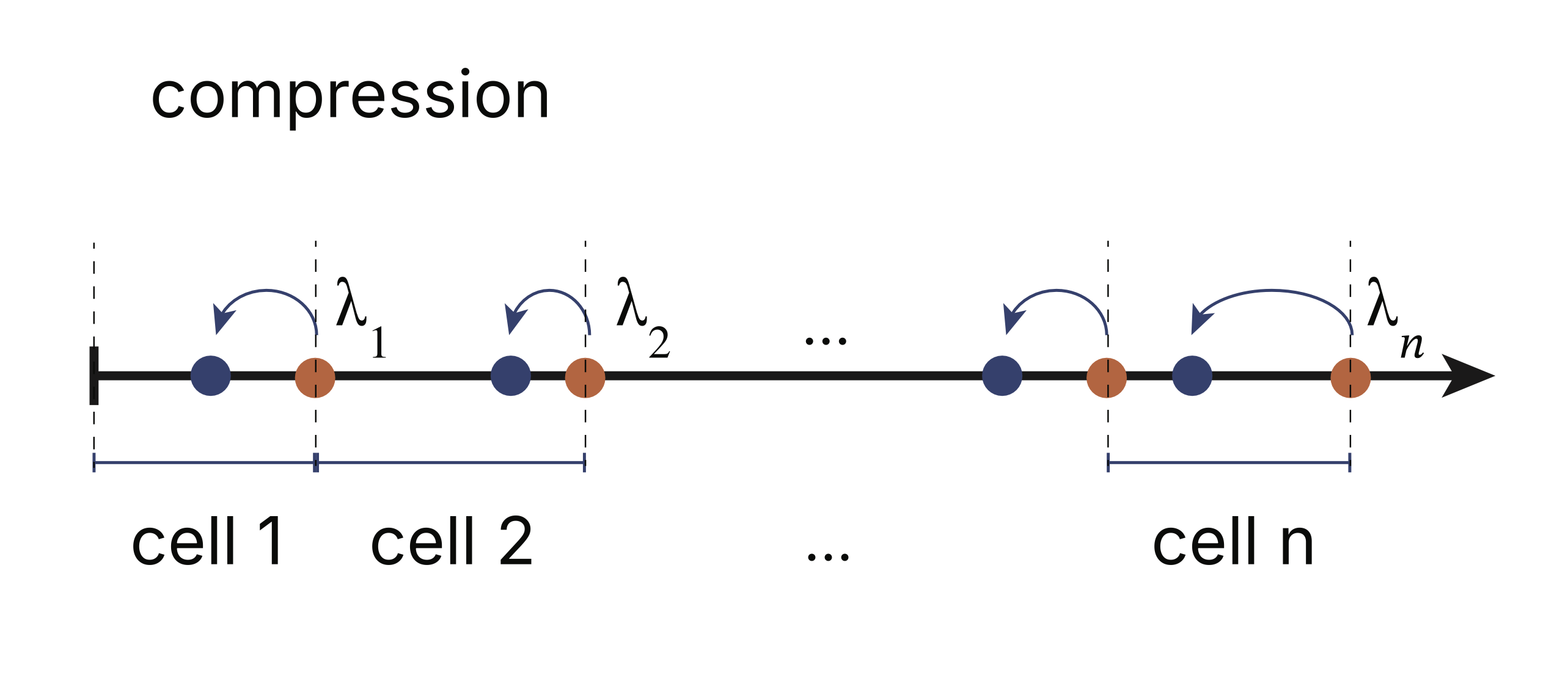
Figure 2: Upon compressing by any finite \(s < 1\), the eigenvalues must always monotonically decrease, always maintaining the interlacing property.

To summarize, if we let the eigenvalues of the original (relatively stretched) matrix be \(\lambda_i^{(s)}\) and those of the compressed system be \(\lambda_i^{(c)}\), we have

\begin{equation} 0 < \lambda_1^{(c)} < \lambda_1^{(s)} < \lambda_2^{(c)} < \ldots < \lambda_n^{(c)} < \lambda_n^{(s)} < \infty, \tag{10}\label{10} \end{equation}

for any generic compression. But of course any compression played in reverse is a stretch, so (\ref{10}) can also be used to characterize what happens under a stretch. It follows that upon any finite stretch, the eigenvalues again interlace, but in the opposite direction: The \(i\)-th eigenvalue will increase, but not so much as to cross the original \((i+1)\)-st eigenvalue. Figure 3 below illustrates these results.

Eigenvalue
interlacing under stretch and compression

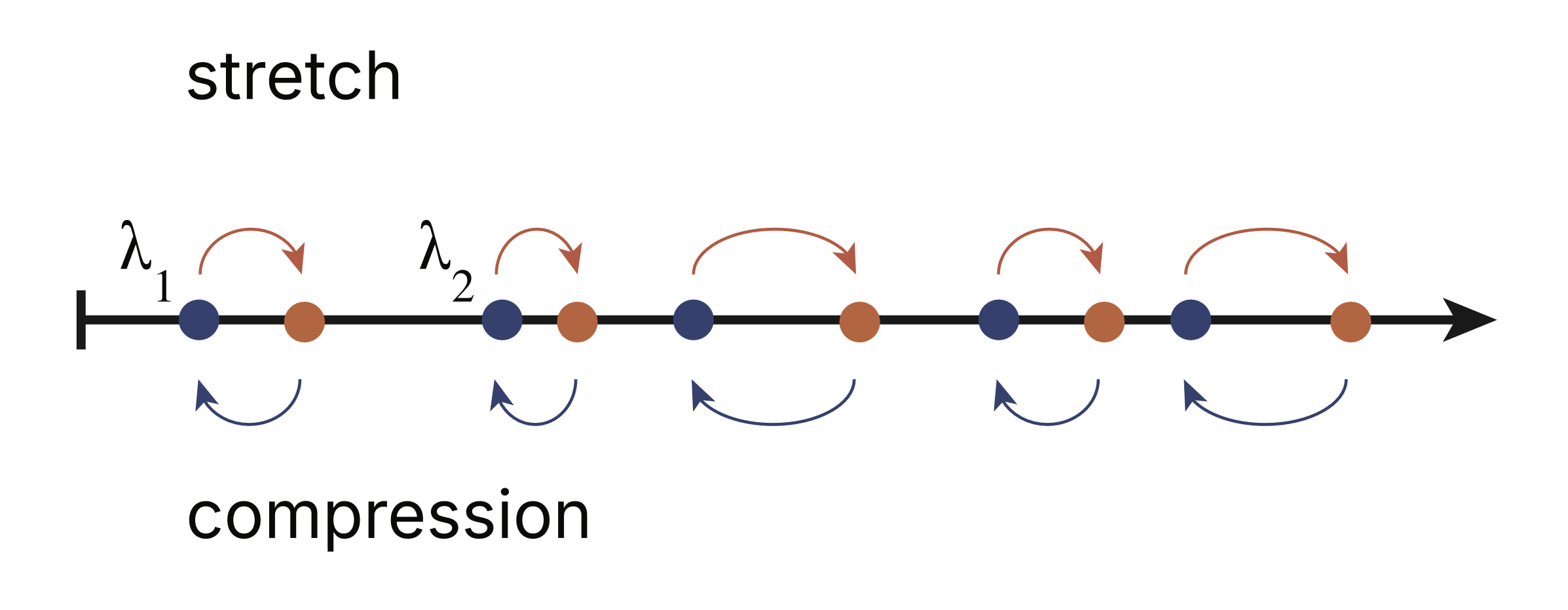
Figure 3: Upon a stretch by \(s > 1\) along a single direction, the eigenvalues generically each increase and maintain their ordering. Further, the \(i\)-th eigenvalue cannot increase beyond the original \(( i+1 )\)-st eigenvalue. Similarly, under a generic compression along a single direction, the eigenvalues each decrease, but without dipping below the original preceding eigenvalues.

Final observations:

Under a generic, single-axis compression or stretch of any finite strength, the eigenvalues interlace the original eigenvalues and maintain their initial order. See Figure 4 below for a numerical example.
Main result: Since any set of compressions and stretches can be carried out via a composition of single-axis compressions and stretches, it follows that in the generic case — where each step's scale direction is not orthogonal to any mode at that point in the composition — the modes will also maintain their order. These results also apply to the non-generic case — see the Appendix.

Figure 4: Here, we plot the eigenvalues of a random five-dimensional covariance matrix \(M(s)\) as a function of \(s\). The eigenvalues never cross one another and satisfy the strict interlacing property. Note that sometimes the eigenvalues appear to bounce off one another. We explain this behavior from a "macroscopic" perspective in the appendix, and detail the microscopics in the companion post.

Summary

We have shown that monotonicity and asymptotic behavior imply that PCA eigenvalues cannot cross under continuous changes in scale, and therefore maintain their ordering. This non-crossing property provides a qualitative picture of how the principal components evolve under changes in scale. E.g., under a strong stretch in one direction, order maintenance tells us that it must be the largest principal component that rotates into the stretch direction. Similarly, under a strong compression, it must be the smallest principal component that rotates into this compression direction — see Figure 1 for an example. Finally, our cell argument provides some insight into how the eigenvalues will change under single-axis scalings, and this can be adapted to understand non-generic cases as well — see the Appendix.

Our result may allay some concern during applications that the results of PCA are sensitive to scale changes. Provided the changes in scale are "generic" and not too large, order maintenance implies that the \(k\)-th mode will more-or-less maintain its character. However, under non-generic scalings with apparent crossings, eigenvalue ordering is maintained only through sudden rotations of the eigenvectors. At such a degeneracy, the two modes effectively swap their character. This should be kept in mind when considering changes of scale of this nature (or nearby cases — again, see the Appendix).

See our companion post for several additional results. There, we derive the asymptotics of strong single-axis scalings and show that any two positive-definite covariance matrices can be connected by a finite sequence of single-axis scalings. That is, the modes of any two positive-definite covariance matrices are connected in the sense discussed here. We also analyze the perturbation equations near a “bounce” and derive a simple expression for the change in determinant under scaling.

Although motivated by PCA, these results apply more generally to arbitrary real symmetric positive-definite matrices, and therefore to a broad class of spectral problems, including covariance matrices of many mechanical systems.

Appendix: Non-generic scaling and instantaneous rotations

Here, we'll first illustrate how our cell argument above can be adapted to anticipate exactly how apparent eigenvalue hopping will occur in the non-generic regime (again, where the scaling direction is orthogonal to some modes). Next, we'll consider what happens as we approach this limit from the generic regime. We'll show that eigenvalue ordering is maintained here via rapid rotations of the modes. If we interpret the non-generic limit as one where similar rotations occur instantaneously, we can then formally say that eigenvalue order maintenance is respected in this regime as well.

Non-generic Apparent Eigenvalue Hopping

The top cell diagram in Figure 5 provides a simple example where eigenvalues can be seen to hop in the non-generic limit. There, we consider a strong compression along a direction orthogonal to the initially smallest eigenvalue mode (we assume the compression direction is not orthogonal to any other mode). From our perturbation equations, this means that \(\lambda_1\) must be fixed throughout. However, we also know that in the limit of a strong compression, one eigenvalue must go to zero and the others must interlace the original eigenvalues. In this case, since \(\lambda_2\) must decrease, we conclude that \(\lambda_1\) and \(\lambda_2\) must be the two (and only two) eigenvalues occupying the first two cells throughout the compression process. Since one of these must go to zero, it follows that \(\lambda_2 \to 0\) as \(s \to 0\), hopping below \(\lambda_1\). The logic then continues as before, with the remaining eigenvalues interlacing — e.g., \(\lambda_3\) must be the only eigenvalue in cell \(3\), etc.

We note that it's also possible to construct simple examples where hopping of intermediate eigenvalues occurs, provided these are orthogonal to the scaling direction. A special case occurs when scaling along a single principal component. In this case, all eigenvalues are frozen except for that corresponding to the scale direction and this can move to any finite value under an appropriate scaling.

Key Observations:

From the perturbation equations (\ref{6}) and (\ref{7}), we see that modes orthogonal to scaling directions cannot move. Strong scalings can then force "apparent" crossings.
As illustrated here, our cell argument can often be adapted to understand qualitatively what happens under non-generic scalings.

Eigenvalue
interlacing breaking down in a non-generic case

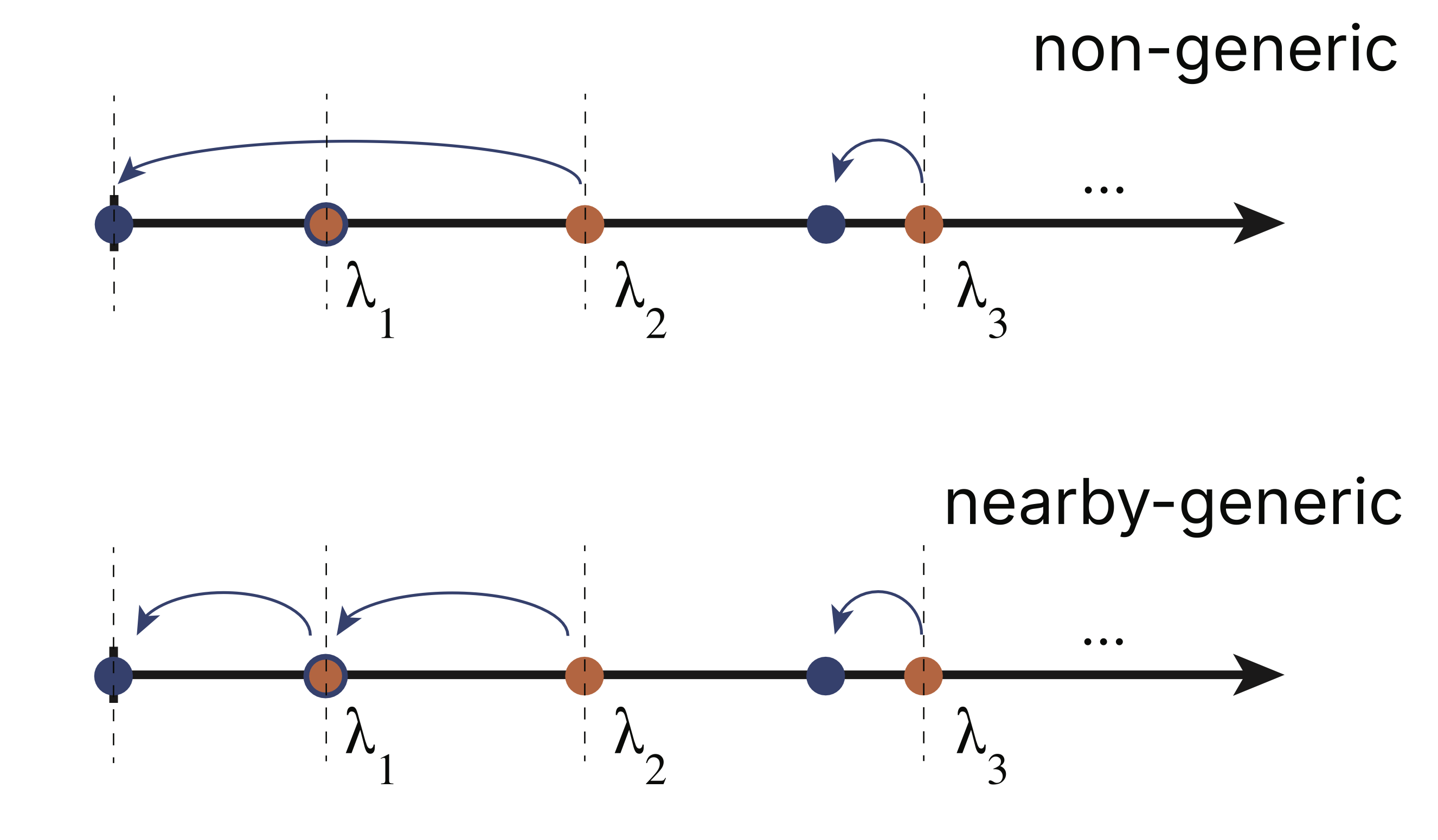
Figure 5: In a non-generic case, some eigenvalues will be frozen and can be hopped. Here, we illustrate what happens under a strong compression orthogonal to the initial lowest mode. In the nearby-generic case, the eigenvalues do not cross. Rather, at the near-crossing, \(\lambda_2\) bounces into \(\lambda_1\), stopping there. The smaller eigenvalue \(\lambda_1\) then continues to zero.

Rapid Rotations Save Order Maintenance

The eigensystem of a matrix is continuous in its components, at least away from any eigenvalue degeneracies. This introduces the question of how we can break order maintenance under a non-generic scale change, but retain it for a nearby generic transformation.

The resolution to the issue can be understood through consideration of the bottom cell diagram of Figure 5. Here, we show what happens for a generic compression very near to the non-generic one considered above it. In this case, the eigenvalues cannot cross, but must ultimately sit very close to those of the compressed non-generic system. By continuity, the eigenvalue locations (ignoring their labels) must approximately match those of the non-generic system for each point in the compression. What must happen in this case then is as follows: Before the apparent crossing, \(\lambda_1\) will hardly budge. However, when \(\lambda_2\) approaches very close to \(\lambda_1\), \(\lambda_1\) will suddenly bounce off and continue towards \(0\), leaving \(\lambda_2\) in its prior place. In words, they'll behave like the balls in a Newton's Cradle toy. This is the only way for the eigenvalues to match in the two systems throughout the continuous compression process.

The eigenvectors must also match throughout. Now, the eigenvector corresponding to \(\lambda_1\) does not change at all in the non-generic scaling. It must similarly barely change as \(\lambda_2\) approaches it in the nearby-generic transformation. For the two systems to continue to match after the bounce, the eigenvector of \(\lambda_2\) must then align with that of \(\lambda_1\) before the bounce. In other words, the two modes must swap orientation right at the bounce in the generic system. This is possible as we have a (near-)degeneracy around the bounce (in a degenerate sub-space we are free to choose any orthogonal basis for the eigensystem — it is this flexibility that allows for the rapid rotation). Figure 6 below illustrates this effect in a simple two-d example.

Key Observations:

A non-generic mode is not affected by scaling if it is orthogonal to the scaling direction. For this reason, it looks like the modes can cross in this case.
However, when considering near-by generic scalings, we see that order maintenance occurs via rapid orientation swaps of the corresponding modes. We can interpret the non-generic crossings as limiting forms of this behavior, also respecting order-stability.

For another view of this behavior, see our companion post, where we work out what happens near a crossing of two eigenvalues via integration of the perturbation equations.

Figure 6: A nearly non-generic scaled system in two dimensions. Here, we have chosen a data set that has one principal component nearly parallel to the \(x\)-axis, the direction along which we scale. In the top panel we show the data and principal components at various values of \(s\). In the bottom we show the eigenvalues at the corresponding values of \(s\). As the two eigenvalues approach each other, we see a rapid rotation of the modes, preventing an eigenvalue crossing.

References

[1] Dobosevych & Hryniv, “Direct and Inverse Spectral Problems for Rank-One Perturbations of Self-adjoint Operators” [link]

Note that interlacing results for rank-one perturbations appear at least as early as the 1960s, but this is the first article we could find that quotes the strict interlacing result we need. However, ChatGPT says this follows directly from the so-called secular equations considered in this sort of analysis.